MCMC integration

General thoughts on integration

Markov chain Monte-Carlo methods entered almost every aspect of the science where simulations are needed. Basically, the problem they solve is to generate random numbers according to some p.d.f. And there are many practical reasons one needs to do that - from finding energy minimum of complex system to numerical integration, which I am going to discuss here.

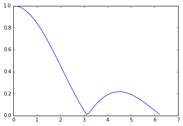
In general, we have to calculate the following: $$\int_{a}^{b} f(x_1,x_2,...,x_N) dx_{1}dx_{2}...dx_{N}$$ When the number of dimensions N is small enough, we can calculate it using standard numerical techniques. How small is small enough? Let's illustrate with $$\int_{0}^{2\pi} \prod_{i=1}^{k} \left| \frac{sin(x_i)}{x_i} \right| dx_i $$ for some values of k. One can easily note the cheating here - integral is easily factorizable and easily computable given value for $\int_{0}^{2\pi} \left| \frac{sin(x)}{x} \right| dx $.

#imports we will need in the future
%matplotlib inline
import numpy as np
import matplotlib.pyplot as plt
import scipy.integrate as integrate
import math
from mpl_toolkits.mplot3d import Axes3D
from matplotlib import cm


#Here is our function in 1d
x=np.arange(0.01,2*math.pi,0.1)
plt.plot(x,abs(np.sin(x)/x))




[<matplotlib.lines.Line2D at 0x12e1b35d0>]

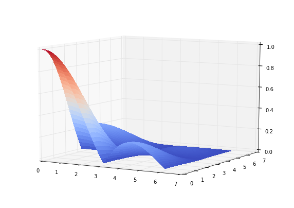
y=np.arange(0.01,2*math.pi,0.1)
mx,my=np.meshgrid(x,y)
z=abs(np.sin(mx)/mx)*abs(np.sin(my)/my)

fig = plt.figure(figsize=(10,7))
ax = fig.gca(projection='3d')

surf = ax.plot_surface(mx,my,z, rstride=1, cstride=1, facecolors=cm.coolwarm(z),shade=False,
                       linewidth=0,antialiased=False)
ax.view_init(elev=10., azim=300)

def f(x1):
    return  abs(np.sin(x1)/x1)
%timeit integrate.quad(f, 0, 2*math.pi)

10000 loops, best of 3: 70.8 µs per loop



def f2(x1,x2):
    return  abs(np.sin(x1)/x1)*abs(np.sin(x2)/x2)
%timeit integrate.nquad(f2, [[0, 2*math.pi],[0, 2*math.pi]])

100 loops, best of 3: 8.67 ms per loop



def f3(x1,x2,x3):
    return  abs(np.sin(x1)/x1)*abs(np.sin(x2)/x2)*abs(np.sin(x3)/x3)
%timeit integrate.nquad(f3, [[0, 2*math.pi],[0, 2*math.pi],[0, 2*math.pi]])

1 loops, best of 3: 769 ms per loop



def f4(x1,x2,x3,x4):
    return  abs(np.sin(x1)/x1)*abs(np.sin(x2)/x2)*abs(np.sin(x3)/x3)*abs(np.sin(x4)/x4)
%time integrate.nquad(f4, [[0, 2*math.pi],[0, 2*math.pi],[0, 2*math.pi],[0, 2*math.pi]])

CPU times: user 1min 5s, sys: 734 ms, total: 1min 5s
Wall time: 1min 6s





(27.29568732908961, 3.019806626980426e-13)




#Check the computation: integral of f4 is just of f1^4
integrate.nquad(f, [[0, 2*math.pi]])[0]**4




27.29568732908961

As we can see, adding a new dimension slows down computation almost 100x! And there is a simple explanation for that: in order to integrate a function you divide interval (in this example $[0,2\pi]$) by N bins (here it's around 100) and then sum across the bins. As a number of dimensions k grows, total number of bins (hence the computation) grows like $N^k$!!! But if you need 10-dimensional integration you have to sum $10^{20}$ values! That's impossible!

Sampling to the resque!

As you can see in 3d plot above, multidimensional functions tend to be more peaked hence lots of computational power is simply wasted in the areas where function is around 0.

Imagine you are discovering a new city. Would you go block-by-block visiting every corner? Probably not. You would rather selected the most interesting places and visited them first. You can even create a list of places, sort it by fun you can get from the place and went through this list. In the real world it is how I do that. But the computer can do even better: go to the place with probability, proportional to the fun you get there. Why? Because if you go by sorted list, you never know how much fun is in the tail of the list (but you know that each entry is less interesting that you are at now, so it's fine in real life). On the other hand, probabilistic solutions allow us to estimate the result at any given point, and improve the result by continuing the process.

Let's get back to the problem of the integration and formulate it in terms of a probabilistic process. $$\int_{a}^{b} f(x) dx = (b-a) \int_{a}^{b} f(x) \frac{1}{b-a} dx = (b-a) \int_{a}^{b} f(x) p(x) dx = (b-a) E_{p}[f] $$ where $p(x) = \frac{1}{b-a}$ is a probability distribution function (pdf) of a uniform random variable. The above line states the following: instead of summing all infinitesimal $f(x) dx$ we can average $f(x)$ along possible values of $x$.

Sometimes on your way

Imagine we can visit the places with higher values of the $f(x_{i})$ more often than to the places with lower $f(x_{i})$. This will allow us to